By the end of this section, you will be able to:
A vector can be multiplied by another vector but may not be divided by another vector. There are two kinds of products of vectors used broadly in physics and engineering. One kind of multiplication is a scalar multiplication of two vectors. Taking a scalar product of two vectors results in a number (a scalar), as its name indicates. Scalar products are used to define work and energy relations. For example, the work that a force (a vector) performs on an object while causing its displacement (a vector) is defined as a scalar product of the force vector with the displacement vector. A quite different kind of multiplication is a vector multiplication of vectors. Taking a vector product of two vectors returns as a result a vector, as its name suggests. Vector products are used to define other derived vector quantities. For example, in describing rotations, a vector quantity called torque is defined as a vector product of an applied force (a vector) and its distance from pivot to force (a vector). It is important to distinguish between these two kinds of vector multiplications because the scalar product is a scalar quantity and a vector product is a vector quantity.
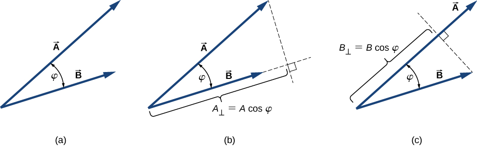
Scalar multiplication of two vectors yields a scalar product.
where [latex] \phi [/latex] is the angle between the vectors (shown in (Figure)). The scalar product is also called the dot product because of the dot notation that indicates it.
For the vectors shown in (Figure), find the scalar product [latex] \overset·\overset [/latex].
In the Cartesian coordinate system, scalar products of the unit vector of an axis with other unit vectors of axes always vanish because these unit vectors are orthogonal:
In these equations, we use the fact that the magnitudes of all unit vectors are one: [latex] |\hat|=|\hat|=|\hat|=1 [/latex]. For unit vectors of the axes, (Figure) gives the following identities:
[latex] \hat·\hat=^=\hat·\hat=^=\hat·\hat=^=1. [/latex]For example, in the rectangular coordinate system in a plane, the scalar x-component of a vector is its dot product with the unit vector [latex] \hat [/latex], and the scalar y-component of a vector is its dot product with the unit vector [latex] \hat [/latex]:
Scalar multiplication of vectors is commutative,
[latex] \overset·\overset=\overset·\overset, [/latex]and obeys the distributive law:
[latex] \overset·(\overset+\overset)=\overset·\overset+\overset·\overset. [/latex]We can use the commutative and distributive laws to derive various relations for vectors, such as expressing the dot product of two vectors in terms of their scalar components.
When the vectors in (Figure) are given in their vector component forms,
[latex] \overset=_\hat+_\hat+_\hat\,\text\,\overset=_\hat+_\hat+_\hat, [/latex]we can compute their scalar product as follows:
Since scalar products of two different unit vectors of axes give zero, and scalar products of unit vectors with themselves give one (see (Figure) and (Figure)), there are only three nonzero terms in this expression. Thus, the scalar product simplifies to
[latex] \overset·\overset=__+__+__. [/latex]We can use (Figure) for the scalar product in terms of scalar components of vectors to find the angle between two vectors . When we divide (Figure) by AB, we obtain the equation for [latex] \text\,\phi [/latex], into which we substitute (Figure):
[latex] \textThree dogs are pulling on a stick in different directions, as shown in (Figure). The first dog pulls with force [latex] <\overset<\to >>_=(10.0\hat-20.4\hat+2.0\hat)\text [/latex], the second dog pulls with force [latex] <\overset<\to >>_=(-15.0\hat-6.2\hat)\text [/latex], and the third dog pulls with force [latex] <\overset<\to >>_=(5.0\hat+12.5\hat)\text [/latex]. What is the angle between forces [latex] <\overset<\to >>_ [/latex] and [latex] <\overset<\to >>_ [/latex]?
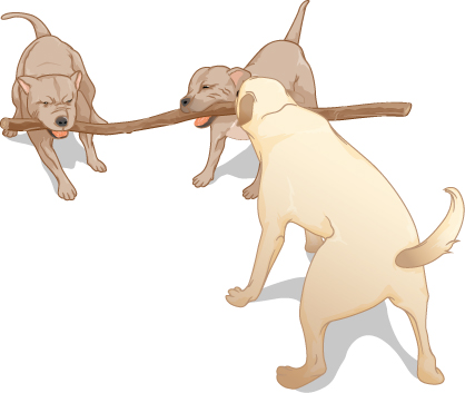
Figure 2.28 Three dogs are playing with a stick.
The components of force vector [latex] <\overset<\to >>_ [/latex] are [latex] _=10.0\,\text [/latex], [latex] _=-20.4\,\text [/latex], and [latex] _=2.0\,\text [/latex], whereas those of force vector [latex] <\overset<\to >>_ [/latex] are [latex] _=-15.0\,\text [/latex], [latex] _=0.0\,\text [/latex], and [latex] _=-6.2\,\text [/latex]. Computing the scalar product of these vectors and their magnitudes, and substituting into (Figure) gives the angle of interest.
[latex] _=\sqrt<_^+_^+_^>=\sqrt^+^>\,\text=16.2\,\text. [/latex] Substituting the scalar components into (Figure) yields the scalar product
Notice that when vectors are given in terms of the unit vectors of axes, we can find the angle between them without knowing the specifics about the geographic directions the unit vectors represent. Here, for example, the +x-direction might be to the east and the +y-direction might be to the north. But, the angle between the forces in the problem is the same if the +x-direction is to the west and the +y-direction is to the south.
Find the angle between forces [latex] <\overset<\to >>_ [/latex] and [latex] <\overset<\to >>_ [/latex] in (Figure).
Show Solution[latex] 131.9\text [/latex]
When force [latex] \overset [/latex] pulls on an object and when it causes its displacement [latex] \overset [/latex], we say the force performs work. The amount of work the force does is the scalar product [latex] \overset·\overset [/latex]. If the stick in (Figure) moves momentarily and gets displaced by vector [latex] \overset=(-7.9\hat-4.2\hat)\,\text [/latex], how much work is done by the third dog in (Figure)?
We compute the scalar product of displacement vector [latex] \overset [/latex] with force vector [latex] <\overset>_=(5.0\hat+12.5\hat)\text [/latex], which is the pull from the third dog. Let’s use [latex] _ [/latex] to denote the work done by force [latex] <\overset>_ [/latex] on displacement [latex] \overset [/latex].
The SI unit of work is called the joule [latex] (\text) [/latex], where 1 J = 1 [latex] \text·\text [/latex]. The unit [latex] \text·\text [/latex] can be written as [latex] ^\text·\text=^\text [/latex], so the answer can be expressed as [latex] _=-0.9875\,\text\approx -1.0\,\text [/latex].
How much work is done by the first dog and by the second dog in (Figure) on the displacement in (Figure)?
Show SolutionVector multiplication of two vectors yields a vector product.
where angle [latex] \phi [/latex], between the two vectors, is measured from vector [latex] \overset [/latex] (first vector in the product) to vector [latex] \overset [/latex] (second vector in the product), as indicated in (Figure), and is between [latex] 0\text [/latex] and [latex] 180\text [/latex].
According to (Figure), the vector product vanishes for pairs of vectors that are either parallel [latex] (\phi =0\text) [/latex] or antiparallel [latex] (\phi =180\text) [/latex] because [latex] \text\,0\text=\text\,180\text=0 [/latex].
The corkscrew right-hand rule is a common mnemonic used to determine the direction of the vector product. As shown in (Figure), a corkscrew is placed in a direction perpendicular to the plane that contains vectors [latex] \overset [/latex] and [latex] \overset [/latex], and its handle is turned in the direction from the first to the second vector in the product. The direction of the cross product is given by the progression of the corkscrew.

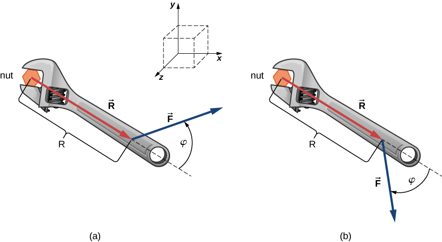
The mechanical advantage that a familiar tool called a wrench provides ((Figure)) depends on magnitude F of the applied force, on its direction with respect to the wrench handle, and on how far from the nut this force is applied. The distance R from the nut to the point where force vector [latex] \overset [/latex] is attached and is represented by the radial vector [latex] \overset [/latex]. The physical vector quantity that makes the nut turn is called torque (denoted by [latex] \overset) [/latex], and it is the vector product of the distance between the pivot to force with the force: [latex] \overset=\overset\,×\,\overset [/latex].
To loosen a rusty nut, a 20.00-N force is applied to the wrench handle at angle [latex] \phi =40\text [/latex] and at a distance of 0.25 m from the nut, as shown in (Figure)(a). Find the magnitude and direction of the torque applied to the nut. What would the magnitude and direction of the torque be if the force were applied at angle [latex] \phi =45\text [/latex], as shown in (Figure)(b)? For what value of angle [latex] \phi [/latex] does the torque have the largest magnitude?
 from the center of the nut. The vector R is the vector from the center of the nut to the location where the force is being applied. The force direction is at an angle phi, measured counterclockwise from the direction of the vector R. Figure b: a wrench grips a nut. A force F is applied to the wrench at a distance R from the center of the nut. The vector R is the vector from the center of the nut to the location where the force is being applied. The force direction is at an angle phi, measured clockwise from the direction of the vector R." width="878" height="482" />
Figure 2.31 A wrench provides grip and mechanical advantage in applying torque to turn a nut. (a) Turn counterclockwise to loosen the nut. (b) Turn clockwise to tighten the nut.
We adopt the frame of reference shown in (Figure), where vectors [latex] \overset [/latex] and [latex] \overset [/latex] lie in the xy-plane and the origin is at the position of the nut. The radial direction along vector [latex] \overset [/latex] (pointing away from the origin) is the reference direction for measuring the angle [latex] \phi [/latex] because [latex] \overset [/latex] is the first vector in the vector product [latex] \overset=\overset\,×\,\overset [/latex]. Vector [latex] \overset [/latex] must lie along the z-axis because this is the axis that is perpendicular to the xy-plane, where both [latex] \overset [/latex] and [latex] \overset [/latex] lie. To compute the magnitude [latex] \tau [/latex], we use (Figure). To find the direction of [latex] \overset [/latex], we use the corkscrew right-hand rule ((Figure)).
For the situation in (a), the corkscrew rule gives the direction of [latex] \overset\,×\,\overset [/latex] in the positive direction of the z-axis. Physically, it means the torque vector [latex] \overset [/latex] points out of the page, perpendicular to the wrench handle. We identify F = 20.00 N and R = 0.25 m, and compute the magnitude using (Figure):
[latex] \tau \,=|\overset\,×\,\overset|=\,RF\,\text\,\phi =(0.25\,\text)(20.00\,\text)\,\text\,40\text=3.21\,\text·\text. [/latex] For the situation in (b), the corkscrew rule gives the direction of [latex] \overset\,×\,\overset [/latex] in the negative direction of the z-axis. Physically, it means the vector [latex] \overset [/latex] points into the page, perpendicular to the wrench handle. The magnitude of this torque is
[latex] \tau \,=|\overset\,×\,\overset|=\,RF\,\text\,\phi =(0.25\,\text)(20.00\,\text)\,\text\,45\text=3.53\,\text·\text. [/latex] The torque has the largest value when [latex] \text\,\phi =1 [/latex], which happens when [latex] \phi =90\text [/latex]. Physically, it means the wrench is most effective—giving us the best mechanical advantage—when we apply the force perpendicular to the wrench handle. For the situation in this example, this best-torque value is [latex] _>=RF=(0.25\,\text)(20.00\,\text)=5.00\,\text·\text [/latex].
When solving mechanics problems, we often do not need to use the corkscrew rule at all, as we’ll see now in the following equivalent solution. Notice that once we have identified that vector [latex] \overset\,×\,\overset [/latex] lies along the z-axis, we can write this vector in terms of the unit vector [latex] \hat [/latex] of the z-axis:
[latex] \overset\,×\,\overset=RF\,\text\,\phi \hat. [/latex]In this equation, the number that multiplies [latex] \hat [/latex] is the scalar z-component of the vector [latex] \overset\,×\,\overset [/latex]. In the computation of this component, care must be taken that the angle [latex] \phi [/latex] is measured counterclockwise from [latex] \overset [/latex] (first vector) to [latex] \overset [/latex] (second vector). Following this principle for the angles, we obtain [latex] RF\,\text\,(+40\text)=+3.2\,\text·\text [/latex] for the situation in (a), and we obtain [latex] RF\,\text\,(-45\text)=-3.5\,\text·\text [/latex] for the situation in (b). In the latter case, the angle is negative because the graph in (Figure) indicates the angle is measured clockwise; but, the same result is obtained when this angle is measured counterclockwise because [latex] +(360\text-45\text)=+315\text [/latex] and [latex] \text\,(+315\text)=\text\,(-45\text) [/latex]. In this way, we obtain the solution without reference to the corkscrew rule. For the situation in (a), the solution is [latex] \overset\,×\,\overset=+3.2\,\text·\text\hat [/latex]; for the situation in (b), the solution is [latex] \overset\,×\,\overset=-3.5\,\text·\text\hat [/latex].
Similar to the dot product ((Figure)), the cross product has the following distributive property:
[latex] \overset\,×\,(\overset+\overset)=\overset\,×\,\overset+\overset\,×\,\overset. [/latex]The distributive property is applied frequently when vectors are expressed in their component forms, in terms of unit vectors of Cartesian axes.
When we apply the definition of the cross product, (Figure), to unit vectors [latex] \hat [/latex], [latex] \hat [/latex], and [latex] \hat [/latex] that define the positive x-, y-, and z-directions in space, we find that
[latex] \hat\,×\,\hat=\hat\,×\,\hat=\hat\,×\,\hat=0. [/latex]All other cross products of these three unit vectors must be vectors of unit magnitudes because [latex] \hat [/latex], [latex] \hat [/latex], and [latex] \hat [/latex] are orthogonal. For example, for the pair [latex] \hat [/latex] and [latex] \hat [/latex], the magnitude is [latex] |\hat\,×\,\hat|=ij\,\text\,90\text=(1)(1)(1)=1 [/latex]. The direction of the vector product [latex] \hat\,×\,\hat [/latex] must be orthogonal to the xy-plane, which means it must be along the z-axis. The only unit vectors along the z-axis are [latex] \text\hat [/latex] or [latex] +\hat [/latex]. By the corkscrew rule, the direction of vector [latex] \hat\,×\,\hat [/latex] must be parallel to the positive z-axis. Therefore, the result of the multiplication [latex] \hat\,×\,\hat [/latex] is identical to [latex] +\hat [/latex]. We can repeat similar reasoning for the remaining pairs of unit vectors. The results of these multiplications are
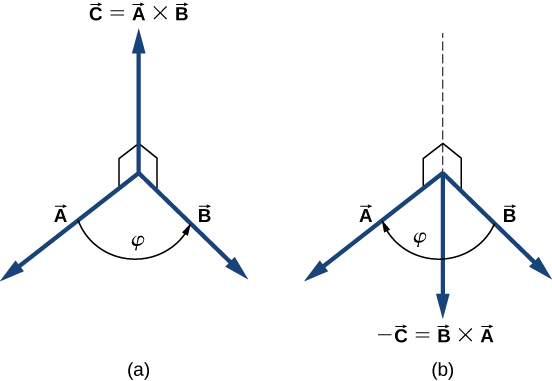
[latex] \\hat\,×\,\hat=+\hat,\\ \hat\,×\,\hat=+\hat,\\ \hat\,×\,\hat=+\hat.\end [/latex]Notice that in (Figure), the three unit vectors [latex] \hat [/latex], [latex] \hat [/latex], and [latex] \hat [/latex] appear in the cyclic order shown in a diagram in (Figure)(a). The cyclic order means that in the product formula, [latex] \hat [/latex] follows [latex] \hat [/latex] and comes before [latex] \hat [/latex], or [latex] \hat [/latex] follows [latex] \hat [/latex] and comes before [latex] \hat [/latex], or [latex] \hat [/latex] follows [latex] \hat [/latex] and comes before [latex] \hat [/latex]. The cross product of two different unit vectors is always a third unit vector. When two unit vectors in the cross product appear in the cyclic order, the result of such a multiplication is the remaining unit vector, as illustrated in (Figure)(b). When unit vectors in the cross product appear in a different order, the result is a unit vector that is antiparallel to the remaining unit vector (i.e., the result is with the minus sign, as shown by the examples in (Figure)(c) and (Figure)(d). In practice, when the task is to find cross products of vectors that are given in vector component form, this rule for the cross-multiplication of unit vectors is very useful.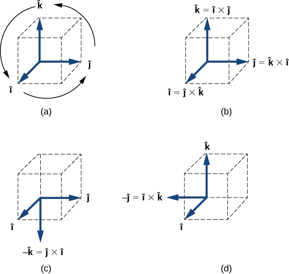
Figure 2.32 (a) The diagram of the cyclic order of the unit vectors of the axes. (b) The only cross products where the unit vectors appear in the cyclic order. These products have the positive sign. (c, d) Two examples of cross products where the unit vectors do not appear in the cyclic order. These products have the negative sign.
When performing algebraic operations involving the cross product, be very careful about keeping the correct order of multiplication because the cross product is anticommutative. The last two steps that we still have to do to complete our task are, first, grouping the terms that contain a common unit vector and, second, factoring. In this way we obtain the following very useful expression for the computation of the cross product:
[latex] \overset=\overset\,×\,\overset=(__-__)\hat+(__-__)\hat+(__-__)\hat. [/latex]In this expression, the scalar components of the cross-product vector are
When finding the cross product, in practice, we can use either (Figure) or (Figure), depending on which one of them seems to be less complex computationally. They both lead to the same final result. One way to make sure if the final result is correct is to use them both.
When moving in a magnetic field, some particles may experience a magnetic force. Without going into details—a detailed study of magnetic phenomena comes in later chapters—let’s acknowledge that the magnetic field [latex] \overset [/latex] is a vector, the magnetic force [latex] \overset [/latex] is a vector, and the velocity [latex] \overset [/latex] of the particle is a vector. The magnetic force vector is proportional to the vector product of the velocity vector with the magnetic field vector, which we express as [latex] \overset=\zeta \overset\,×\,\overset [/latex]. In this equation, a constant [latex] \zeta [/latex] takes care of the consistency in physical units, so we can omit physical units on vectors [latex] \overset [/latex] and [latex] \overset [/latex]. In this example, let’s assume the constant [latex] \zeta [/latex] is positive.
A particle moving in space with velocity vector [latex] \overset=-5.0\hat-2.0\hat+3.5\hat [/latex] enters a region with a magnetic field and experiences a magnetic force. Find the magnetic force [latex] \overset [/latex] on this particle at the entry point to the region where the magnetic field vector is (a) [latex] \overset=7.2\hat-\hat-2.4\hat [/latex] and (b) [latex] \overset=4.5\hat [/latex]. In each case, find magnitude F of the magnetic force and angle [latex] \theta [/latex] the force vector [latex] \overset [/latex] makes with the given magnetic field vector [latex] \overset [/latex].
First, we want to find the vector product [latex] \overset\,×\,\overset [/latex], because then we can determine the magnetic force using [latex] \overset=\zeta \overset\,×\,\overset [/latex]. Magnitude F can be found either by using components, [latex] F=\sqrt<_^+_^+_^> [/latex], or by computing the magnitude [latex] |\overset\,×\,\overset| [/latex] directly using (Figure). In the latter approach, we would have to find the angle between vectors [latex] \overset [/latex] and [latex] \overset [/latex]. When we have [latex] \overset [/latex], the general method for finding the direction angle [latex] \theta [/latex] involves the computation of the scalar product [latex] \overset·\overset [/latex] and substitution into (Figure). To compute the vector product we can either use (Figure) or compute the product directly, whichever way is simpler.
The components of the velocity vector are [latex] _=-5.0 [/latex], [latex] _=-2.0 [/latex], and [latex] _=3.5 [/latex].
(a) The components of the magnetic field vector are [latex] _=7.2 [/latex], [latex] _=-1.0 [/latex], and [latex] _=-2.4 [/latex]. Substituting them into (Figure) gives the scalar components of vector [latex] \overset=\zeta \overset\,×\,\overset [/latex]:
Thus, the magnetic force is [latex] \overset=\zeta (8.3\hat+13.2\hat+19.4\hat) [/latex] and its magnitude is
[latex] F=\sqrt_^+_^+_^>=\zeta \sqrt^+^+^>=24.9\zeta . [/latex] To compute angle [latex] \theta [/latex], we may need to find the magnitude of the magnetic field vector,
[latex] \overset·\overset=__+__+__=(8.3\zeta )(7.2)+(13.2\zeta )(-1.0)+(19.4\zeta )(-2.4)=0. [/latex] Now, substituting into (Figure) gives angle [latex] \theta [/latex]:
Hence, the magnetic force vector is perpendicular to the magnetic field vector. (We could have saved some time if we had computed the scalar product earlier.)
(b) Because vector [latex] \overset=4.5\hat [/latex] has only one component, we can perform the algebra quickly and find the vector product directly:
[latex] \begin\hfill \overset& =\zeta \overset\,×\,\overset=\zeta (-5.0\hat-2.0\hat+3.5\hat)\,×\,(4.5\hat)\hfill \\ & =\zeta [(-5.0)(4.5)\hat\,×\,\hat+(-2.0)(4.5)\hat\,×\,\hat+(3.5)(4.5)\hat\,×\,\hat]\hfill \\ & =\zeta [-22.5(\text\hat)-9.0(+\hat)+0]=\zeta (-9.0\hat+22.5\hat).\hfill \end [/latex] The magnitude of the magnetic force is
[latex] \overset·\overset=__+__+__=(-9.0\zeta )(0)+(22.5\zeta )(0)+(0)(4.5)=0, [/latex] the magnetic force vector [latex] \overset [/latex] is perpendicular to the magnetic field vector [latex] \overset [/latex].
Even without actually computing the scalar product, we can predict that the magnetic force vector must always be perpendicular to the magnetic field vector because of the way this vector is constructed. Namely, the magnetic force vector is the vector product [latex] \overset=\zeta \overset\,×\,\overset [/latex] and, by the definition of the vector product (see (Figure)), vector [latex] \overset [/latex] must be perpendicular to both vectors [latex] \overset [/latex] and [latex] \overset [/latex].